SDSR Home Page
Home page for the SDSR project
HW1
CA2
Identify two other papers (say Q and R) chosen for class presentation by other groups. You team will peer-review presentations prepared by other teams on Q and R.
Paper Q: Foundation Models for Scientific Discovery and Innovation
Paper R: A Survey on Uncertainty Quantiifcation Methods for Deep Learning
CA3
Submit an electronic copy (plain text or other standard format files) of the narrative and slides. Use file formats (e.g. powerpoint, pdf), which are supported widely by browsers. Electronic copy will be linked to the web-page for the course to make those available to the audience. The written critique should be about 1500 ~ 2000 words long and the oral presentation should consist of about 10 slides addressing the following questions:
- Problem statement: Formally define the problem addressed in the paper. Briefly explain the significance of the problem in context of our course.
- List the major contributions of the paper. Which do you think is most significant and why?
- What are the key concepts behind the approach in this paper. Provide simple explanations of those. Also provide a couple of simple exercises for the audience to check their undersanding of the key concepts.
- What is the validation methodology (e.g. case studies, statistical hypothesis testing, proofs, simulation) used in this paper? Describe the strengths and weaknesses of the methodology. Why did authors choose this methodology?
- List the assumptions made by the authors. Critique an assumption that you believe is unreasonable. What is the impact of removing this unreasonable assumption on the solution proposed by the authors?
Written Critique:
The paper we reviewed together, and made the above slides for, is an updated software library used for training Graph Neural Networks (GNNs). PyG 2.0 is a July 2025 framework that was an update to the existing PyTorch Geometric (PyG) library. The intent of the update was to improve PyG’s utility for research-based training, particularly for complex research projects. They mainly attempted this by introducing mechanisms for the users to provide instructions during pre-processing that PyG can follow during training. While they also provided new tensor formats to utilize behind the scenes, the main contribution of PyG 2.0 is the user-based plug-and-play approach that PyG did not have before.
For example, users can now specify how they want their features and graphs stored during pre-processing to help alleviate message passing. Message passing can also be alleviated by the users by taking advantage of: a new EdgeIndex tensor that holds node indices in a sparse Coordinate Format; a caching mechanism to allow fast coversions to compressed sparse column/row formats; and kernel fusion to enable multiple operations in a single kernel. PyG 2.0 also natively supports heterogenous graphs for multiple node and edge types by leverageing goruped and segmented matrix multiplications by utilizing libraries such as CUTLASS.
Explainability is also expanded upon with an Explainer and CaptumExplainer modules. The Explainer module takes in user inputs to create masks for features and nodes that are weighted by each component’s contributions to the prediction model. During training, the masks are manuplated alongside the data and returned as data that can help build an explanation model of the finalized trained model. The authors state that with Explainer, researchers only need to focus on the challenge of building explainer algorithms instead of trying to extrapolate from a trained foundation model.
The CaptumExplainer module creates a wrapper around a PyG GNN to provide the needed inputs for the Captum library to take advantage of. This helps overcome the challenge of taking a GNN with non-differentiable inputs and translating it to node features with an edge-level soft mask needed for most Captum applications. The authors claim that with CaptumExplainer, any GNN input can now be utilized by Captum to get feature information and structural properties.
The authors list multiple instances in which PyG 2.0 could see practical applications. Two that they went in depth with are Relational Deep Learning (RDL) and Large Language Models (LLMs). Since PyG 2.0 natively supports heterogeneous graphs, the end-to-end RDL process for multi-modal data, recommender systems that are GNN-based, and training tables are supported. Offering felxibile loading routines such as ground-truth tables are an additional utility for RDL. LLMs benefit from PyG by utilizing text-attributed graphs and through supported Retrieval Augmented Generration (RAG) techniques. The authors cite an effective 16-32% accuracy improvement using GNN+LLM-based Graph RAG from an NVIDIA article.
The remaining list of applications in section 3.3 inlcude: drug discovery using chemistry foundation models with GNN from PyG; weather forecasting and traffic behavior prediction with large spatial graphs; combinatorial optimizatiom problems, and a dominant paradigm for solving them; bot, community and fake news detection in social networks; handling unstructured data in computer vision; and open-source ecosystems such as Quiver, AutoGL, DIG, PyGOD, FedGraphNN and Relbench. All applications had multiple sources listed to back the authors’ claims up. No further information was provided beyond a brief summary in the conclusion, and an acknowledgement of NVIDIA and Intel for supporting the published work.
At the risk of oversimplifying the framework’s new utilities, consider a user of PyG had a particular project for training in mind with a given dataset, and had an idea of how the training data should be organized in advance. In the prior iteration of PyG, they had to provide the data and hope that PyG organized the training process efficiently. Given certain training requirements or data types and no ability to tailor the training nor create an explanation model for it, high computation costs would be inevitable. The created model would also not provide explanatory data to train with, opening the door for potential black box problems. With PyG 2.0, they can now specify how message passing during training should be carried out and how the data’s structure should be set up for training. If they want an explanation of the model, they can also create one using specific commands with the Explainer module.
Let us consider a more specific example: a bank wants to create an LLM to interact with potential customers and determine if they should get a loan or increased credit. The local government taxes them for exceeding electricity usage to any company that uses LLMs, has strict laws against racial profiling, and requires that all LLMs that interact with the public or corporate sector are not black boxes if the actions taken from them have a publicly noticeable effect. PyG 2.0 will allow the bank to organize the LLM training in a way that better guarantees them minimum energy waste and thus avoids higher taxes on top of their expected increased electric bill. The plug-and-play interface allows the bank to also remove racial bias from the training as best as they can. The Explainer module can also provide the dataset needed to determine, with CaptumExplainer, the best record possible of how the LLM model could have racial bias in it. The bank can utilize these modules to make corrections before deploying the model to the public or to defend the model in court should it be investigated for it. Alternatively, the government also now has a tool to investigate the model themselves.
To validate that PyG 2.0 was more efficient for message passing, they ran several tests using different GNN architectures with a compiled version of their software against a baseline. They also tested a pruning ‘trim’ method for subraph sampling tests using the previous test as a baseline. When it came to applications in research or real-world applications, however, they only discussed how PyG 2.0 supports them in section 3. The paper explains the framework quite well, but they leave the reader to infer or even make their own code based on the README they provided in their linked GitHub page.
Allowing the readers to be able to access their updated framework allows those with a more hands-on approach to learning access to test their own refinements or questions. This method is also very useful for enabling readers to both build on their framework or contrast it with their pre-existing code in the prior PyG framework. On the other hand, without a tutorial on how to write their code, the user will need a background with Python, PyTorch, and the previous PyG to be able to test the new framework. Without that experience, the user is required to learn that code on their own. They also do not provide rigorous mathematical justifications themselves. They only utilize citations with the presumption they back up their claims. It is efficient to read their main points and arguments, but extensive work to check their assumptions. They most likely chose this route since they are providing an update to a coding library and have a code-savvy audience in mind.
It is possible that they are presuming all the underlying math for organizing their new frameworks’ applications checks out. For example, they provide a formula for the callback mechanism used by the Explainer module and then simplify how the callback mechanism interacts with the training in two sentences. They provide a citation for the reader to follow up on the math underlying the interactions, and the variable used to represent the callback mechanism is not provided in their illustration of the Explainer module (Figure 2). This can be problematic if there was a complication with the callback mechanism’s interactions with training that the paper ignored. For example, if it turned out that the callback mechanism’s weight function only worked if it was scaled down to the range [0,1] then the callback mechanism could risk being compromised by data underflow. Anyone that just read the paper and did not follow the citations up would need to experiment with PyG 2.0 to rule out this weakness on their own. We did not utilize their code on our own, so we cannot state for certain if this is the case.
We think the most unreasonable assumption the authors made is that anyone that reads their paper will be able to follow up with experimentating with their code. Most of the applications the authors state PyG 2.0 is compatible with will involve having computers that are able to hold and train with large sets of data in a reasonable time frame. PyG also must be compatible with the hardware available to the readers. Requiring NVIDIA RAPIDS (the framework for CuGraph intergration) prevents users that cannot support NVIDIA applications on their computers from testing on their own. The authors also leave it to the readers to do their own research on how to construct LLMs or RDL apparatuses with PyG to confirm their conjectures in section 3.
CP1
Define possible questions, i.e. preliminary proposal outlining areas of interest based on the examination of course material. The question should be related to a topic covered in the course but not completely addressed by the papers in the reading list.
- What kinds of spatial indexing techniques would be most useful for real-time ingestion and querying of geospatial data streams generated by drones?
- What database architectures best support local vs remote processing for autonomous drone fleets performing large-scale mapping tasks?
- How can uncertainty in drone sensor data be modeled and queried efficiently within spatial database systems?
- What spatial data management techniques enable efficient coordiantion and collision avoidance among multiple drones operating in shared 3D space?
- How can incremental spatial updates from drones be integrated into existing GIS systems without requiring full recomputation of spatial indexes or derived products?
DA1
Each group will be assigned a week of class notes to work on. Generate alternative text for the first 5 images in the slide deck. To do this, download the slide deck from the “Slides” column of the Notes table for the assigned week. To generate alternative text for an image in the slide deck, simply download the image and upload it to the Image Accessibility Generator. To insert an alternative text, right click an image in the slide and select “Edit Alt Text …” in the drop down menu in Microsoft Powerpoint.
The annotated slides can be found here. The images with the generated alt text can be found below.
Images and their corresponding Alt Text Image Breakdown Outputs:
 Long Description:
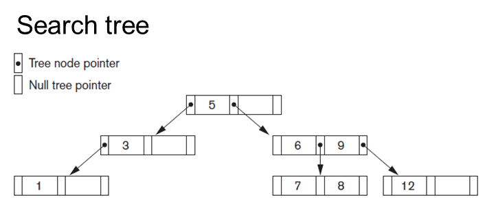
The image illustrates a binary search tree diagram. At the top level, the word “Search tree” is displayed. Below it, there are two legends: a filled circle indicating a “Tree node pointer” and an empty circle indicating a “Null tree pointer.” The tree structure begins with the root node labeled “5,” connected by arrows pointing to its left and right child nodes. The left child node, labeled “3,” further points to its own left child, labeled “1.” On the right side of the root, the node “6” points to its right child, labeled “9.” The node “9” has two children: “7” on the left and “8” on the right. The node “9” also points to the value “12” on the far right. Each node is represented by a small rectangle with two or three compartments, indicating the tree pointer structure.
Alt-text:
Diagram of a binary search tree with nodes labeled 1, 3, 5, 6, 7, 8, 9, and 12.
Transcribed Text:
Search tree Tree node pointer Null tree pointer
“Long Description:
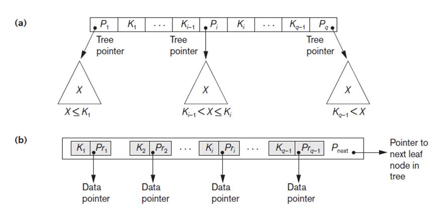
The image contains two diagrams labeled as (a) and (b), depicting hierarchical structures likely related to data organization in trees. Diagram (a) illustrates a tree node structure with boxes aligned horizontally. Boxes labeled ( P_1, K_1 ) are followed by ellipses indicating more elements (( K_{i-1}, P_i, K_i )), ending with ( K_{q-1}, P_q ). Below each of these labels are triangles marked ( X ), connected by arrows labeled “Tree pointer,” with conditions like ( X \leq K_1 ) and ( K_i < X ). Diagram (b) depicts a sequence of boxes labeled ( K_1, P_{r1} ), continuing with ellipses until ( K_{q-1}, P_{r(q-1)} ), ending with ( P_{\text{next}} ). Arrows beneath indicate “Data pointer” relating to each series of ( K ) and ( Pr ) pairs. An arrow labeled “Pointer to next leaf node in tree” points right from ( P_{\text{next}} ).
Alt-text:
Two diagrams showing hierarchical data structures with labeled nodes and pointers for tree organization.
Transcribed Text:
(a) Tree pointer; X ≤ K1; Ki−1 < X ≤ Ki; Kq−1 < X (b) Data pointer; Pointer to next leaf node in tree
Long Description:
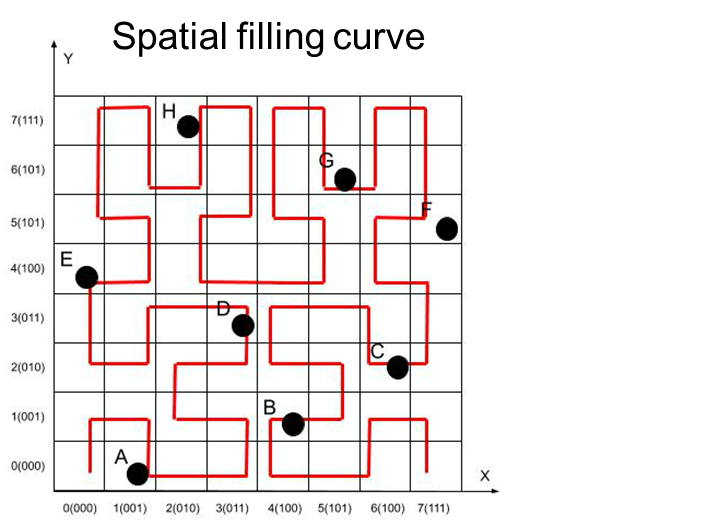
The image shows a grid with both x and y axes labeled from 0 to 7. The grid contains a red, continuous line representing a spatial filling curve, winding through small squares in a pattern across the entire grid. Several black dots are plotted along the path of the curve at specific coordinates. Letters label each dot from A to H. The overall path of the curve appears to fill the grid in a systematic way. The top of the image contains the title “Spatial filling curve.”
Alt-text:
Spatial filling curve on a grid with labeled axes, featuring a red line and black dots labeled A to H.
Transcribed Text:
Spatial filling curve A, B, C, D, E, F, G, H X-axis: 0(000), 1(001), 2(010), 3(011), 4(100), 5(101), 6(110), 7(111) Y-axis: 0(000), 1(001), 2(010), 3(011), 4(100), 5(101), 6(110), 7(111)
Long Description:
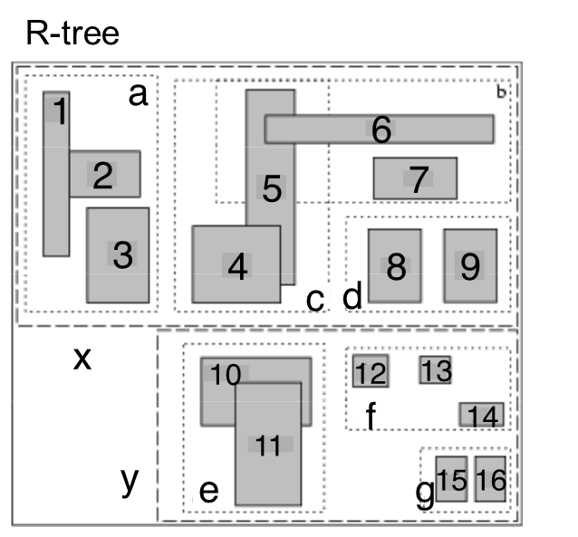
The image is a diagram labeled “R-tree,” depicting a hierarchical structure of rectangular nodes and sub-rectangles, presumably representing spatial data. The layout is divided into two main sections, separated by a dashed horizontal line labeled “x” and “y.” Each section contains several labeled sub-rectangles. In the top section, labeled “a,” “b,” “c,” and “d,” there are nine smaller rectangles labeled from 1 to 9. The bottom section contains rectangles labeled “e,” “f,” “g,” and sub-rectangles numbered 10 through 16. The rectangles are shaded, with some overlapping or nested within larger dashed borders that group them into categories.
Alt-text:
Diagram of an R-tree with rectangles labeled 1 to 16, organized in two sections and various groups.
Transcribed Text:
R-tree a b c d e f g x y 1 2 3 4 5 6 7 8 9 10 11 12 13 14 15 16
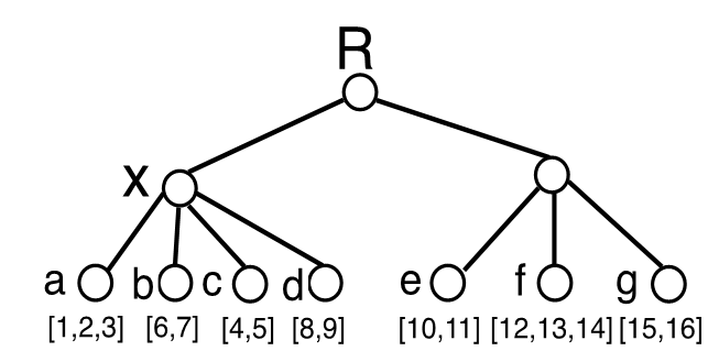
Long Description:
The image depicts a binary tree structure with nodes connected by lines, illustrating a hierarchical arrangement. At the top is the node labeled “R,” which branches into two nodes labeled “X” and another node (“e”) on the right side. The node “X” further branches into four nodes labeled “a,” “b,” “c,” and “d.” On the right side of “R,” the node “e” connects to two other nodes labeled “f” and “g.” Each leaf node contains numbers within brackets, representing data associated with each node. The connections form a clear and structured pattern typical of tree data structures.
Alt-text:
Illustration of a binary tree structure with labeled nodes.
Transcribed Text:
R, X, a [1,2,3], b [6,7], c [4,5], d [8,9], e [10,11], f [12,13,14], g [15,16].